Section 3.5.1: Systems Reducible to Iteration in a Single Unknown

It is frequently possible, by analysing the structure of a set of equations, typically by creating an incidence or occurrence table to see which equations appear in which unknowns, to discover that what looks like a large set of simultaneous equations can in fact be solved by a combination of rearrangement, and by iterating in a single variable. Both of these techniques have already been covered individually; we will now see how they can be combined to solve more complicated problems.

Illustrative Example

Consider the 4 equations in unknowns w, x, y, z:

log(w) + 3 = 0

w + 5 x² - y - 4 = 0

x + log( y) = 0

w + x + y - z^0.5 + 10 = 0

Without performing any analysis of the equation, we might suppose that it would be necessary to guess the values of all 4 unknowns and iterate on all of them simultaneously, using techniques which we have not yet discussed.

However, experience with problems involving direct solution where we could reorder and rearrange sets of equations to solve without any iteration whatsoever, tells us that we should look more closely at the equations.

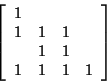
Here is an incidence matrix for the equations as written above in the rows and the variables in order w, x, y, z in the columns.

It is obvious that the first equation contains only the unknown w and so can immediately be solved after rearranging to the formula:

w = exp(-3) = 0.0498

w is now known and so is no longer a variable. We can if we wish remove the w column from the incidence table and look at the remaining 3 variable problem. In particular, w is no longer an unknown in the second equation, which now effectively contains only x and y. However, all the other equations also contain at least both x and y and so it is not possible to go any further with `direct' solution.

In fact, it can be seen that the second and third equations now contain both x and y and only these unknowns. They must be solved simultaneously, and for this purpose could be rewritten with the value of w substituted in as:

0.0498 + 5 x² - y - 4 = 0

x + log( y) = 0

Although the above equations will have to be solved simultaneously somehow, once we have done this and determined values for x and y it can be seen that in the last equation there now remains only the single unknown, z. This can then be determined by rearrangement:

z = (10 + w + x + y)º

Summary so Far

We can divide the equations in a set of algebraic equations into three categories:

The `head' of the equation set which is a subset of the equations which can be solved directly by rearrangement. In this case the head contains only one equation, which may be solved for w, but in some cases the whole set may be solved this way.
The `partition' which is a subset of the equations which must be solved simultaneously. In this case there are 2 equations in the partition which require simultaneous solution for x and y.
A `tail' of the set which can be solved by simple rearrangement once the partition has been solved. In this case there is only one equation in the tail, to be solved for z.

We can use the incidence matrix to help identify these subsets.

Start to find the `head' by looking for any row (equation) with only one nonzero entry (variable). This can be solved on its own. Remove the variable (column) from the set and look for any other single variables. We can reorder the `head' subset of the table to be lower triangular as is the case for any set of equations which can be solved directly.
Start to find the `tail' by looking for any variable (column) which only occurs in a single equation (row). This variable can be solved for once all others in the problem have been determined. Remove the equation (row) and look for any other variables which now occur only in one equation. The table for the tail may also be made lower triangular.
What is left after the head and tail are removed must be the partition. This has an incidence matrix which cannot be made lower triangular no matter how rows and columns are interchanged.

Solving the Partition

Consider the two `partition' equations: 0.0498 + 5 x² - y - 4 = 0

x + log( y) = 0

Suppose we knew x and rearranged the first equation to give y:

y = 0.0498 + 5 x² - 4

If we then substituted the values of x and y into the LHS of the second equation then it should equal zero.

However, if we only guess the value of x, but nonetheless calculate y and substitute it into the second equation, the latter will evaluate to zero if we have chosen the correct value of x. In effect the two equations if rearranged appropriately and treated in sequence:

y = 0.0498 + 5 x² - 4

f = x + log( y)

effectively result in the evaluation of a single function of x:

f(x) = x + log[0.0498 + 5 x² - 4]

This is just a single equation in x and can be solved using any suitable single equation solving method. However the function evaluation is carried out in two steps rather than in one. Note that we do not actually make the substitution shown above. Doing the evaluation in two steps saves us the need to carry out any algebra other than the rearrangement of the first equation.

This method of solving sets of equations is called `tearing' and the single variable x for which we solve is called the `tear variable'. In a more complicated system of equations it may be necessary to tear, i.e. guess and iterate on, more than one tear variable, and so it will not be possible to use the simple solution schemes which have been described for single unknowns. However, many practically useful problems may be reduced to iteration in a single variable.

Inspection of the incidence matrix for the partition will show how many tear variables are needed for a given problem: this is equal to the number of variables (columns) which have nonzero table entries above the diagonal of the matrix. For this example it can be seen that there is only one.

Next - Section 3.5.2: Additional Notes
Return to Section 3 Index